Introduction
The centrimpact package provides tools for analyzing and
visualizing community-engaged research metrics based on the CEnTR*IMPACT
framework (Price, 2024). This framework quantifies four critical
dimensions of community-engaged research that go beyond traditional
academic metrics:
- Alignment - Shared vision between researchers and partners
- Cascade Effects - Ripple effects across social networks
- Dynamics - Quality of partnership processes
- Indicators - Traditional academic productivity markers
This vignette demonstrates the basic workflow for analyzing each dimension and creating publication-ready visualizations.
Installation
# Install from GitHub
devtools::install_github("CENTR-IMPACT/centrimpact-review")Analyzing Project Alignment
The Alignment Score (Sa) quantifies consensus between researchers and community partners across four key areas: Goals, Values, Roles, and Resources. Higher scores indicate stronger shared vision.
Generate and Analyze Data
# Generate example alignment data
alignment_data <- generate_alignment_data(seed = 36)

# View the structure
head(alignment_data)
#>   alignment       role rating
#> 1     Goals researcher   0.53
#> 2     Goals researcher   0.85
#> 3     Goals researcher   0.37
#> 4     Goals researcher   0.97
#> 5     Goals researcher   0.64
#> 6     Goals    partner   0.42

# Analyze alignment
alignment_results <- analyze_alignment(alignment_data)

# View results
print(alignment_results)
#> $table
#>     alignment partner researcher
#> 1  Activities   0.545       0.86
#> 2 Empowerment   0.780       0.70
#> 3       Goals   0.565       0.64
#> 4    Outcomes   0.765       0.77
#> 5     Outputs   0.730       0.69
#> 6   Resources   0.790       0.68
#> 7       Roles   0.730       0.71
#> 8      Values   0.735       0.56
#>
#> $plot_data
#>      alignment       role    rating min_val max_val
#> 1   Activities    partner 0.5450000   0.545   0.545
#> 2   Activities researcher 0.8600000   0.860   0.860
#> 3  Empowerment    partner 0.7800000   0.780   0.780
#> 4  Empowerment researcher 0.7000000   0.700   0.700
#> 5        Goals    partner 0.5650000   0.565   0.565
#> 6        Goals researcher 0.6400000   0.640   0.640
#> 7     Outcomes    partner 0.7650000   0.765   0.765
#> 8     Outcomes researcher 0.7700000   0.770   0.770
#> 9      Outputs    partner 0.7300000   0.730   0.730
#> 10     Outputs researcher 0.6900000   0.690   0.690
#> 11   Resources    partner 0.7900000   0.790   0.790
#> 12   Resources researcher 0.6800000   0.680   0.680
#> 13       Roles    partner 0.7300000   0.730   0.730
#> 14       Roles researcher 0.7100000   0.710   0.710
#> 15      Values    partner 0.7350000   0.735   0.735
#> 16      Values researcher 0.5600000   0.560   0.560
#> 17  Activities    overall 0.6846167      NA      NA
#> 18 Empowerment    overall 0.7389181      NA      NA
#> 19       Goals    overall 0.6013319      NA      NA
#> 20    Outcomes    overall 0.7674959      NA      NA
#> 21     Outputs    overall 0.7097183      NA      NA
#> 22   Resources    overall 0.7329393      NA      NA
#> 23       Roles    overall 0.7199306      NA      NA
#> 24      Values    overall 0.6415606      NA      NA
#>
#> $icc
#>  Single Score Intraclass Correlation
#>
#>    Model: twoway
#>    Type : agreement
#>
#>    Subjects = 8
#>      Raters = 2
#>    ICC(A,1) = -0.383
#>
#>  F-Test, H0: r0 = 0 ; H1: r0 > 0
#>   F(7,6.99) = 0.515 , p = 0.799
#>
#>  95%-Confidence Interval for ICC Population Values:
#>   -1.05 < ICC < 0.473
#>
#> $alignment_score
#> [1] 0.3829787
#>
#> attr(,"class")
#> [1] "alignment_analysis"
Visualize with Slopegraph
The slopegraph shows how researcher and partner ratings compare across domains:
# Create slopegraph visualization
plot_slopegraph <- visualize_alignment(alignment_results)
print(plot_slopegraph)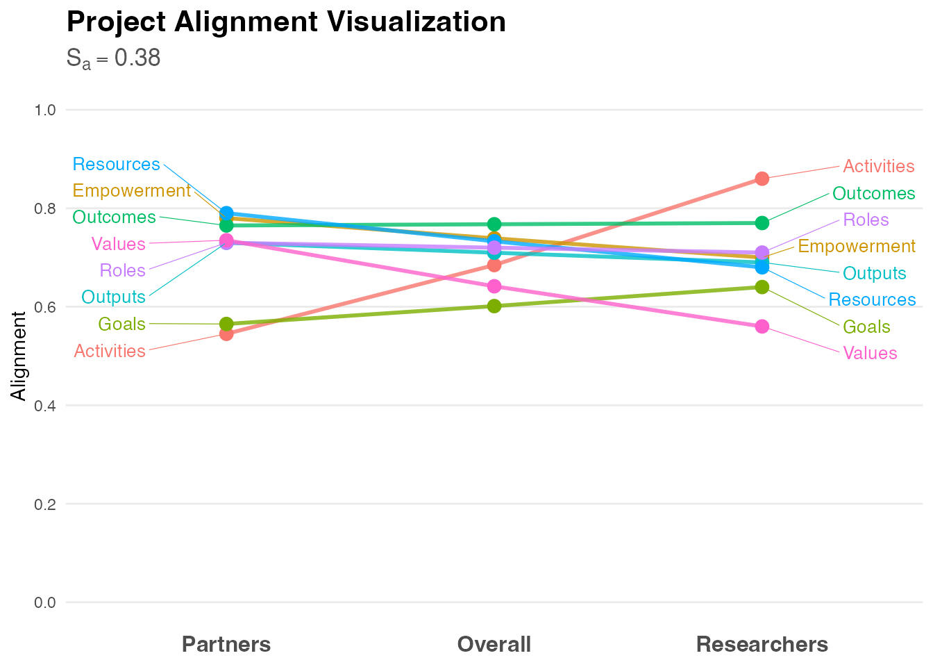
Visualize with Abacus Plot
The abacus plot provides an alternative view of alignment patterns:
# Create abacus plot
plot_abacus <- visualize_abacus(alignment_results)
print(plot_abacus)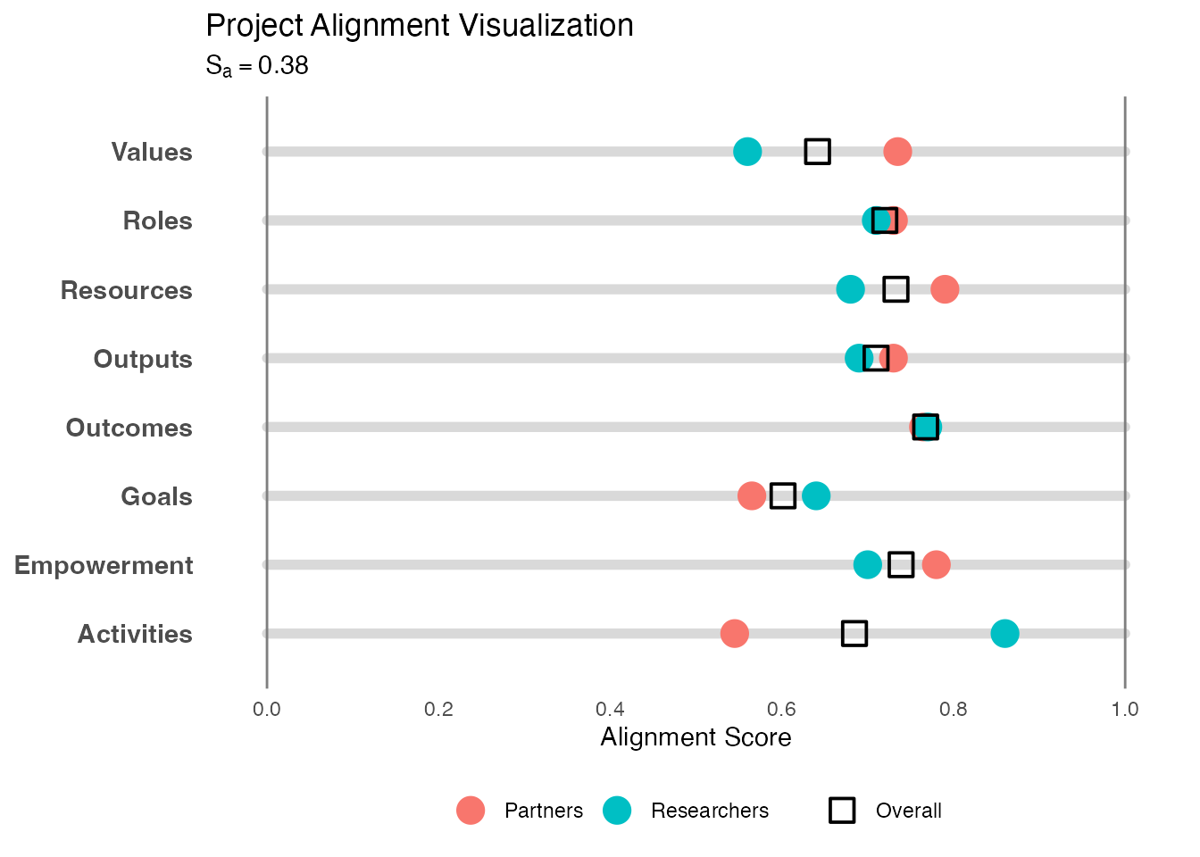
Analyzing Cascade Effects
The Cascade Effects Score (Sc) quantifies how information and power distribute across three degrees of separation from core participants, based on social network analysis principles.
Generate and Analyze Data
# Generate example cascade data (returns a one-row survey parameter frame)
cascade_data <- generate_cascade_data(seed = 36)

# View the structure
print(cascade_data)
#>   cascade_d1_people_1_1 cascade_d1_people_2_1 cascade_d2_people_1_1
#> 1                     6                     4                     4
#>   cascade_d2_people_2_1 cascade_d2_stats_1 cascade_d2_stats_2 cascade_d3_people
#> 1                     4               0.06               0.29                 2
#>   cascade_d3_stats_1 cascade_d3_stats_2
#> 1               0.04               0.08

# Analyze cascade effects
cascade_results <- analyze_cascade(cascade_data)
#> Running full exact analysis (~356 expected edges).

# View results
print(cascade_results)
#> $summary
#> # A tibble: 3 × 9
#>   layer count gamma layer_knitting layer_bridging layer_channeling
#>   <int> <int> <dbl>          <dbl>          <dbl>            <dbl>
#> 1     1    10  0.9           0.462         0.866             0.768
#> 2     2    40  0.5           0.311         0.671             0.525
#> 3     3    80  0.45          0.304         0.0214            0.117
#> # ℹ 3 more variables: layer_reaching <dbl>, layer_score <dbl>,
#> #   layer_number <chr>
#>
#> $node_data
#>     name layer gamma  knitting  bridging  channeling     reaching
#> 1      1     1  0.90 0.2310191 0.8914286 0.761128885 8.687130e-01
#> 2      2     1  0.90 0.4410191 0.8914286 0.842286629 8.746834e-01
#> 3      3     1  0.90 0.8610191 0.8914286 0.817723573 8.568997e-01
#> 4      4     1  0.90 0.4410191 0.7714286 0.623909285 8.531427e-01
#> 5      5     1  0.90 0.4410191 0.8914286 0.801594718 8.872156e-01
#> 6      6     1  0.90 0.2310191 1.0000000 1.000000000 1.000000e+00
#> 7      7     1  0.90 0.2310191 0.8914286 0.805660476 8.726926e-01
#> 8      8     1  0.90 0.4410191 0.8914286 0.818248382 9.083834e-01
#> 9      9     1  0.90 0.4410191 0.7714286 0.693940714 8.399535e-01
#> 10    10     1  0.90 0.8610191 0.7714286 0.518150963 8.705867e-01
#> 11    11     2  0.50 0.2476336 0.7714286 0.647774315 2.357223e-01
#> 12    12     2  0.50 0.3456865 0.6285714 0.436476124 6.629096e-02
#> 13    13     2  0.50 0.3058511 0.6285714 0.436476124 6.629096e-02
#> 14    14     2  0.50 0.3959871 0.6285714 0.436476124 1.397907e-01
#> 15    15     2  0.50 0.3931732 0.7714286 0.686983766 2.082751e-01
#> 16    16     2  0.50 0.3006751 0.6285714 0.503779818 6.696343e-02
#> 17    17     2  0.50 0.2570330 0.6285714 0.503779818 6.696343e-02
#> 18    18     2  0.50 0.4005983 0.6285714 0.503779818 6.696343e-02
#> 19    19     2  0.50 0.2613928 0.6285714 0.482505536 6.494104e-02
#> 20    20     2  0.50 0.4600816 0.6285714 0.482505536 6.494104e-02
#> 21    21     2  0.50 0.2310191 0.7714286 0.659675143 9.909114e-02
#> 22    22     2  0.50 0.2910092 0.6285714 0.482505536 1.384408e-01
#> 23    23     2  0.50 0.2752293 0.6285714 0.433499082 1.227962e-01
#> 24    24     2  0.50 0.2722332 0.7714286 0.679989784 2.192931e-01
#> 25    25     2  0.50 0.3678516 0.6285714 0.433499082 9.829632e-02
#> 26    26     2  0.50 0.2832792 0.6285714 0.433499082 4.929651e-02
#> 27    27     2  0.50 0.3310426 0.6285714 0.468701335 6.819949e-02
#> 28    28     2  0.50 0.2909445 0.7714286 0.643832394 2.135120e-01
#> 29    29     2  0.50 0.2722332 0.6285714 0.468701335 6.819949e-02
#> 30    30     2  0.50 0.2440603 0.6285714 0.468701335 6.819949e-02
#> 31    31     2  0.50 0.2837613 0.7714286 0.683679382 2.136962e-01
#> 32    32     2  0.50 0.2310191 0.6285714 0.525892539 9.012599e-02
#> 33    33     2  0.50 0.3192071 0.7714286 0.699558217 2.032272e-01
#> 34    34     2  0.50 0.3482623 0.6285714 0.525892539 1.391258e-01
#> 35    35     2  0.50 0.2310191 0.6285714 0.472492272 6.506078e-02
#> 36    36     2  0.50 0.3707362 0.6285714 0.472492272 6.506078e-02
#> 37    37     2  0.50 0.2486168 0.7714286 0.670800035 2.009685e-01
#> 38    38     2  0.50 0.2740614 0.6285714 0.472492272 1.140606e-01
#> 39    39     2  0.50 0.3289623 0.6285714 0.486892710 1.179417e-01
#> 40    40     2  0.50 0.3107460 0.6285714 0.486892710 6.894189e-02
#> 41    41     2  0.50 0.2775804 0.7714286 0.696971196 2.634384e-01
#> 42    42     2  0.50 0.2810420 0.6285714 0.513714144 8.263349e-02
#> 43    43     2  0.50 0.3081590 0.6285714 0.497918175 4.979089e-02
#> 44    44     2  0.50 0.5810191 0.6285714 0.497918175 6.612416e-02
#> 45    45     2  0.50 0.3401606 0.6285714 0.532764957 1.134621e-01
#> 46    46     2  0.50 0.2722332 0.7714286 0.709770950 1.859441e-01
#> 47    47     2  0.50 0.2551971 0.7714286 0.476873322 1.336329e-01
#> 48    48     2  0.50 0.4402654 0.6285714 0.362452981 8.687832e-02
#> 49    49     2  0.50 0.2381512 0.7714286 0.578073191 2.715398e-01
#> 50    50     2  0.50 0.2697450 0.6285714 0.326726583 6.491119e-02
#> 51    51     3  0.45 0.3381864 0.0000000 0.131129373 1.997112e-02
#> 52    52     3  0.45 0.5352767 0.0000000 0.131129373 7.509591e-02
#> 53    53     3  0.45 0.3294841 0.0000000 0.063899810 3.374881e-03
#> 54    54     3  0.45 0.2310191 0.0000000 0.063899810 3.374881e-03
#> 55    55     3  0.45 0.3768237 0.0000000 0.063899810 2.174981e-02
#> 56    56     3  0.45 0.2594669 0.0000000 0.063899810 3.374881e-03
#> 57    57     3  0.45 0.2456855 0.0000000 0.063899810 3.374881e-03
#> 58    58     3  0.45 0.2636547 0.0000000 0.063899810 3.374881e-03
#> 59    59     3  0.45 0.3619790 0.0000000 0.163670063 2.005613e-02
#> 60    60     3  0.45 0.4626586 0.0000000 0.163670063 5.155601e-02
#> 61    61     3  0.45 0.2840413 0.0000000 0.119837217 3.475457e-03
#> 62    62     3  0.45 0.3689594 0.0000000 0.119837217 2.239746e-01
#> 63    63     3  0.45 0.2508059 0.0000000 0.119837217 3.475457e-03
#> 64    64     3  0.45 0.2351713 0.0000000 0.119837217 3.475457e-03
#> 65    65     3  0.45 0.2883897 0.0000000 0.119837217 3.475457e-03
#> 66    66     3  0.45 0.3463329 0.0000000 0.119837217 3.475457e-03
#> 67    67     3  0.45 0.2310191 0.0000000 0.102277803 3.171421e-03
#> 68    68     3  0.45 0.3094132 0.0000000 0.102277803 3.171421e-03
#> 69    69     3  0.45 0.2689447 0.0000000 0.102277803 3.171421e-03
#> 70    70     3  0.45 0.3089000 0.0000000 0.102277803 3.171421e-03
#> 71    71     3  0.45 0.3221706 0.0000000 0.143719974 5.597495e-02
#> 72    72     3  0.45 0.2330344 0.0000000 0.143719974 1.187512e-02
#> 73    73     3  0.45 0.2805217 0.0000000 0.102277803 3.171421e-03
#> 74    74     3  0.45 0.2829164 0.0000000 0.102277803 3.171421e-03
#> 75    75     3  0.45 0.3751205 0.0000000 0.060882947 1.102496e-01
#> 76    76     3  0.45 0.3198483 0.0000000 0.060882947 0.000000e+00
#> 77    77     3  0.45 0.2851901 0.0000000 0.155036536 2.122241e-02
#> 78    78     3  0.45 0.2696205 0.0000000 0.155036536 2.122241e-02
#> 79    79     3  0.45 0.4376948 0.0000000 0.060882947 4.409983e-02
#> 80    80     3  0.45 0.2720390 0.0000000 0.060882947 0.000000e+00
#> 81    81     3  0.45 0.2310191 0.0000000 0.060882947 0.000000e+00
#> 82    82     3  0.45 0.3070574 0.0000000 0.060882947 0.000000e+00
#> 83    83     3  0.45 0.2975953 0.0000000 0.089854402 3.643575e-03
#> 84    84     3  0.45 0.3437040 0.0000000 0.089854402 6.979332e-02
#> 85    85     3  0.45 0.2405363 0.0000000 0.131242377 2.080677e-02
#> 86    86     3  0.45 0.3626060 0.0000000 0.131242377 2.080677e-02
#> 87    87     3  0.45 0.3420384 0.0000000 0.089854402 3.643575e-03
#> 88    88     3  0.45 0.3759121 0.0000000 0.089854402 3.643575e-03
#> 89    89     3  0.45 0.3685673 0.0000000 0.089854402 4.774341e-02
#> 90    90     3  0.45 0.2428298 0.0000000 0.089854402 3.643575e-03
#> 91    91     3  0.45 0.2649346 0.0000000 0.160670387 2.486598e-02
#> 92    92     3  0.45 0.2623500 0.0000000 0.160670387 2.486598e-02
#> 93    93     3  0.45 0.2679133 0.0000000 0.135126102 7.813157e-03
#> 94    94     3  0.45 0.3046883 0.0000000 0.135126102 7.813157e-03
#> 95    95     3  0.45 0.2855057 0.0000000 0.174915858 1.654167e-02
#> 96    96     3  0.45 0.2310191 0.0000000 0.174915858 1.654167e-02
#> 97    97     3  0.45 0.3208963 0.0000000 0.135126102 7.813157e-03
#> 98    98     3  0.45 0.2590785 0.0000000 0.135126102 7.813157e-03
#> 99    99     3  0.45 0.3377790 0.0000000 0.093742606 3.186992e-03
#> 100  100     3  0.45 0.5460191 0.0000000 0.093742606 3.258688e-02
#> 101  101     3  0.45 0.2643055 0.0000000 0.093742606 3.186992e-03
#> 102  102     3  0.45 0.3114527 0.0000000 0.093742606 3.186992e-03
#> 103  103     3  0.45 0.2767999 0.0000000 0.153964632 1.254068e-02
#> 104  104     3  0.45 0.2310191 0.0000000 0.153964632 1.254068e-02
#> 105  105     3  0.45 0.2463240 0.0000000 0.093742606 3.186992e-03
#> 106  106     3  0.45 0.3511262 0.0000000 0.093742606 3.186992e-03
#> 107  107     3  0.45 0.2850611 0.0000000 0.106196421 3.753944e-03
#> 108  108     3  0.45 0.2634972 0.0000000 0.106196421 3.753944e-03
#> 109  109     3  0.45 0.3252998 0.0000000 0.106196421 3.753944e-03
#> 110  110     3  0.45 0.3200912 0.0000000 0.106196421 6.990369e-02
#> 111  111     3  0.45 0.3311492 0.0000000 0.172816865 2.497635e-02
#> 112  112     3  0.45 0.2432690 0.0000000 0.172816865 2.497635e-02
#> 113  113     3  0.45 0.4420753 0.4285714 0.357393635 4.619592e-02
#> 114  114     3  0.45 0.3265094 0.0000000 0.140590359 6.627147e-03
#> 115  115     3  0.45 0.2868704 0.0000000 0.118513655 8.037924e-05
#> 116  116     3  0.45 0.2496596 0.0000000 0.118513655 8.037924e-05
#> 117  117     3  0.45 0.2944472 0.0000000 0.118513655 8.037924e-05
#> 118  118     3  0.45 0.3049567 0.0000000 0.118513655 8.037924e-05
#> 119  119     3  0.45 0.4012790 0.4285714 0.386875194 1.355279e-01
#> 120  120     3  0.45 0.2876536 0.0000000 0.159022532 3.092891e-03
#> 121  121     3  0.45 0.2764653 0.4285714 0.397474387 6.008921e-02
#> 122  122     3  0.45 0.3105502 0.0000000 0.194629420 1.985487e-02
#> 123  123     3  0.45 0.3138596 0.0000000 0.006477468 8.969169e-03
#> 124  124     3  0.45 0.2860127 0.0000000 0.006477468 8.969169e-03
#> 125  125     3  0.45 0.2865619 0.0000000 0.010122479 4.722804e-04
#> 126  126     3  0.45 0.2310191 0.0000000 0.010122479 4.722804e-04
#> 127  127     3  0.45 0.3048490 0.0000000 0.080393449 1.725641e-02
#> 128  128     3  0.45 0.2400665 0.0000000 0.080393449 1.725641e-02
#> 129  129     3  0.45 0.2474648 0.4285714 0.142613763 3.990934e-02
#> 130  130     3  0.45 0.2310191 0.0000000 0.000000000 3.246517e-03
#>     composite_score
#> 1        0.68807239
#> 2        0.76235442
#> 3        0.85676773
#> 4        0.67237492
#> 5        0.75531450
#> 6        0.80775477
#> 7        0.70020019
#> 8        0.76476985
#> 9        0.68658547
#> 10       0.75529632
#> 11       0.47563969
#> 12       0.36925626
#> 13       0.35929740
#> 14       0.40020633
#> 15       0.51496517
#> 16       0.37499745
#> 17       0.36408692
#> 18       0.39997824
#> 19       0.35935270
#> 20       0.40902491
#> 21       0.44030349
#> 22       0.38513173
#> 23       0.36502400
#> 24       0.48573617
#> 25       0.38205461
#> 26       0.34866156
#> 27       0.37412871
#> 28       0.47992937
#> 29       0.35942637
#> 30       0.35238315
#> 31       0.48814135
#> 32       0.36890226
#> 33       0.49835526
#> 34       0.41046301
#> 35       0.34928589
#> 36       0.38421516
#> 37       0.47295347
#> 38       0.37229642
#> 39       0.39059203
#> 40       0.37378802
#> 41       0.50235463
#> 42       0.37649027
#> 43       0.37110987
#> 44       0.44340821
#> 45       0.40373976
#> 46       0.48484421
#> 47       0.40928297
#> 48       0.37954203
#> 49       0.46479818
#> 50       0.32248855
#> 51       0.12232173
#> 52       0.18537549
#> 53       0.09918970
#> 54       0.07457345
#> 55       0.11561833
#> 56       0.08168540
#> 57       0.07824004
#> 58       0.08273236
#> 59       0.13642630
#> 60       0.16947117
#> 61       0.10183849
#> 62       0.17819281
#> 63       0.09352965
#> 64       0.08962099
#> 65       0.10292560
#> 66       0.11741140
#> 67       0.08411708
#> 68       0.10371562
#> 69       0.09359848
#> 70       0.10358730
#> 71       0.13046639
#> 72       0.09715738
#> 73       0.09649274
#> 74       0.09709140
#> 75       0.13656325
#> 76       0.09518282
#> 77       0.11536226
#> 78       0.11146985
#> 79       0.13566941
#> 80       0.08323049
#> 81       0.07297551
#> 82       0.09198509
#> 83       0.09777331
#> 84       0.12583793
#> 85       0.09814636
#> 86       0.12866379
#> 87       0.10888410
#> 88       0.11735252
#> 89       0.12654127
#> 90       0.08408196
#> 91       0.11261774
#> 92       0.11197158
#> 93       0.10271313
#> 94       0.11190690
#> 95       0.11924082
#> 96       0.10561915
#> 97       0.11595888
#> 98       0.10050444
#> 99       0.10867716
#> 100      0.16808714
#> 101      0.09030878
#> 102      0.10209557
#> 103      0.11082631
#> 104      0.09938110
#> 105      0.08581339
#> 106      0.11201396
#> 107      0.09875286
#> 108      0.09336190
#> 109      0.10881253
#> 110      0.12404783
#> 111      0.13223560
#> 112      0.11026555
#> 113      0.31855906
#> 114      0.11843173
#> 115      0.10136610
#> 116      0.09206342
#> 117      0.10326031
#> 118      0.10588769
#> 119      0.33806339
#> 120      0.11244226
#> 121      0.29065007
#> 122      0.13125861
#> 123      0.08232656
#> 124      0.07536484
#> 125      0.07428917
#> 126      0.06040346
#> 127      0.10062472
#> 128      0.08442909
#> 129      0.21463983
#> 130      0.05856640
#>
#> $cascade_score
#> [1] 0.6689556
#>
#> $topology_score
#> [1] 0.2310191
#>
#> $mode
#> [1] "full"
#>
#> $estimated_edges
#> [1] 356.2
#>
#> $scale_used
#> [1] 1
#>
#> $n_runs
#> [1] 1
#>
#> attr(,"class")
#> [1] "cascade_analysis"
Visualize with Racetrack Plot
The radial bar chart (“racetrack plot”) shows distribution across network degrees:
# Create cascade visualization
plot_cascade <- visualize_cascade(cascade_results)
print(plot_cascade)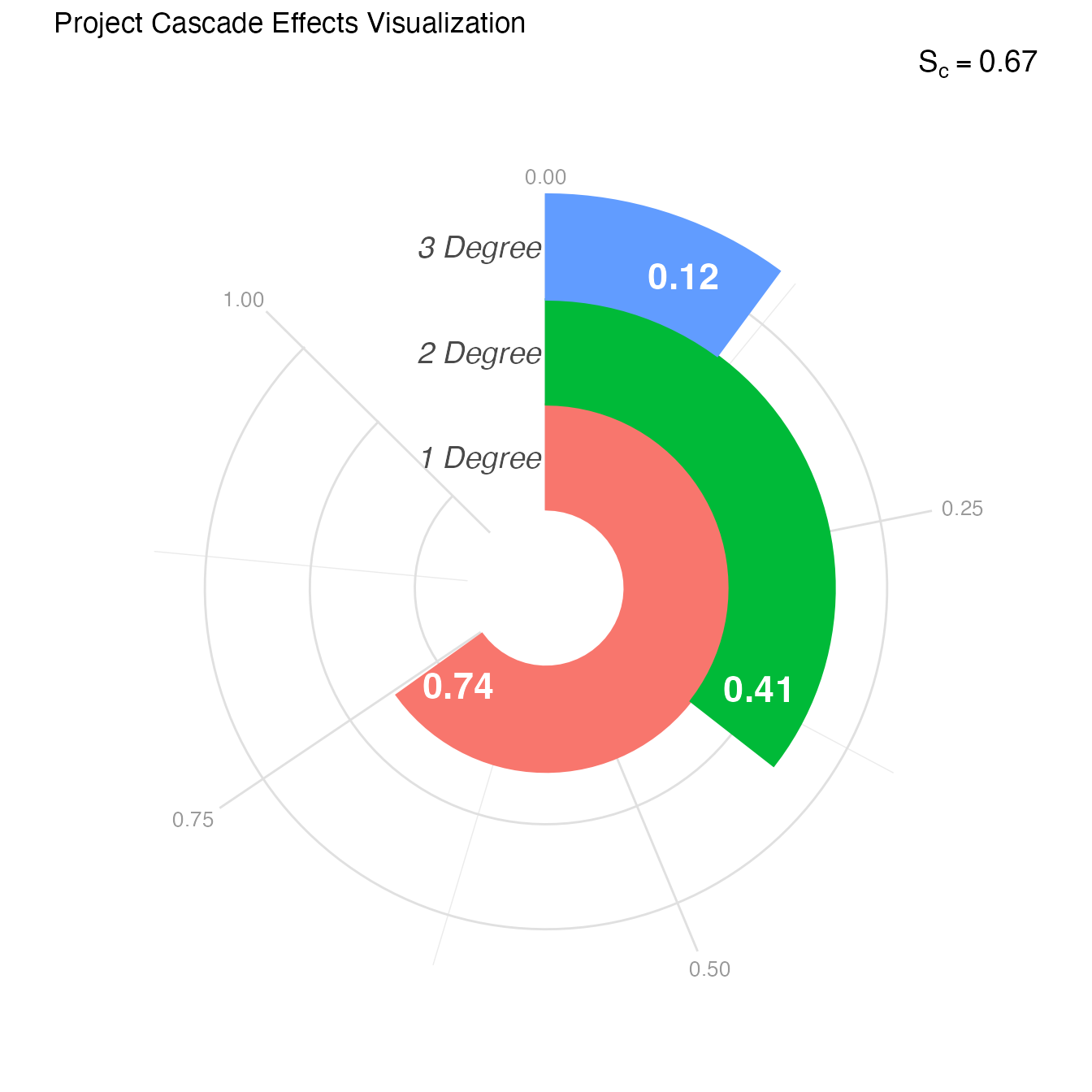
Analyzing Project Dynamics
The Project Dynamics Score (Sd) quantifies how well a project follows Community-Based Participatory Research (CBPR) principles (Wallerstein & Duran, 2010; Wallerstein et al., 2020).
Generate and Analyze Data
# Generate example dynamics data
dynamics_data <- generate_dynamics_data(seed = 36)

# View the structure
head(dynamics_data)
#>     domain dimension salience weight
#> 1 Contexts Challenge      0.2   0.78
#> 2 Contexts Challenge      0.8   0.84
#> 3 Contexts Challenge      0.6   0.95
#> 4 Contexts Challenge      0.4   1.00
#> 5 Contexts Challenge      1.0   1.00
#> 6 Contexts Diversity      0.4   0.84

# Analyze project dynamics
dynamics_results <- analyze_dynamics(dynamics_data)

# View results
print(dynamics_results)
#> $dynamics_df
#> # A tibble: 103 × 7
#>    domain dimension salience weight dimension_value dimension_score domain_score
#>    <chr>  <chr>        <dbl>  <dbl>           <dbl>           <dbl>        <dbl>
#>  1 Conte… Challenge      0.2   0.78           0.156            0.47         0.45
#>  2 Conte… Challenge      0.8   0.84           0.672            0.47         0.45
#>  3 Conte… Challenge      0.6   0.95           0.57             0.47         0.45
#>  4 Conte… Challenge      0.4   1              0.4              0.47         0.45
#>  5 Conte… Challenge      1     1              1                0.47         0.45
#>  6 Conte… Diversity      0.4   0.84           0.336            0.42         0.45
#>  7 Conte… Diversity      0.2   0.9            0.18             0.42         0.45
#>  8 Conte… Diversity      0.6   0.78           0.468            0.42         0.45
#>  9 Conte… Diversity      1     0.78           0.78             0.42         0.45
#> 10 Conte… Diversity      0.8   0.78           0.624            0.42         0.45
#> # ℹ 93 more rows
#>
#> $domain_df
#> # A tibble: 5 × 2
#>   domain       domain_score
#>   <ord>               <dbl>
#> 1 Contexts             0.45
#> 2 Partnerships         0.46
#> 3 Research             0.44
#> 4 Learning             0.46
#> 5 Outcomes             0.44
#>
#> $dynamics_score
#> [1] 0.9893333
#>
#> attr(,"class")
#> [1] "dynamics_analysis"
Visualize with Rose Chart
The rose chart displays dynamics across CBPR dimensions:
# Create dynamics visualization
plot_dynamics <- visualize_dynamics(dynamics_results)
print(plot_dynamics)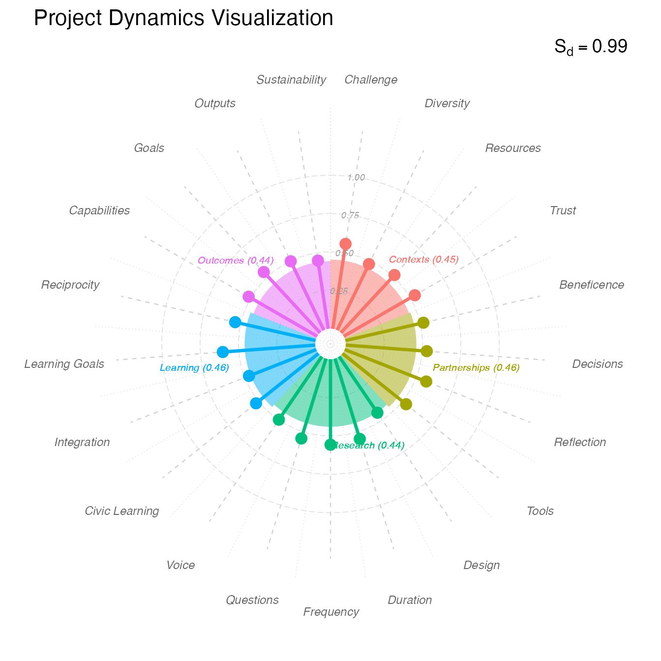
Visualizing Project Indicators
Project Indicators capture traditional academic metrics. These require no separate analysis function as they represent direct counts.
Generate and Visualize Data
# Generate example indicators data
indicators_data <- generate_indicators_data(seed = 36)

# View the structure
head(indicators_data)
#>              indicator value
#> 1   Community Partners    20
#> 2     Engagement Hours    13
#> 3   Individuals Served     2
#> 4 Infrastructure Tools     3
#> 5      Output Products    24
#> 6    Students Involved    22

# Create horizontal bubble chart
plot_indicators <- visualize_indicators(indicators_data)
print(plot_indicators)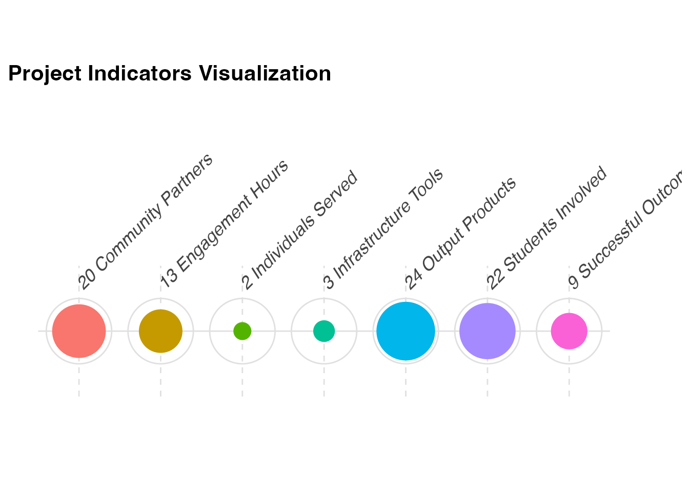
Customizing Visualizations
All visualization functions return ggplot2 objects,
allowing for further customization:
library(ggplot2)

# Customize alignment plot
plot_slopegraph +
  labs(title = "Researcher-Partner Alignment",
       subtitle = "Community Health Equity Project") +
  theme_minimal() +
  theme(plot.title = element_text(face = "bold", size = 14))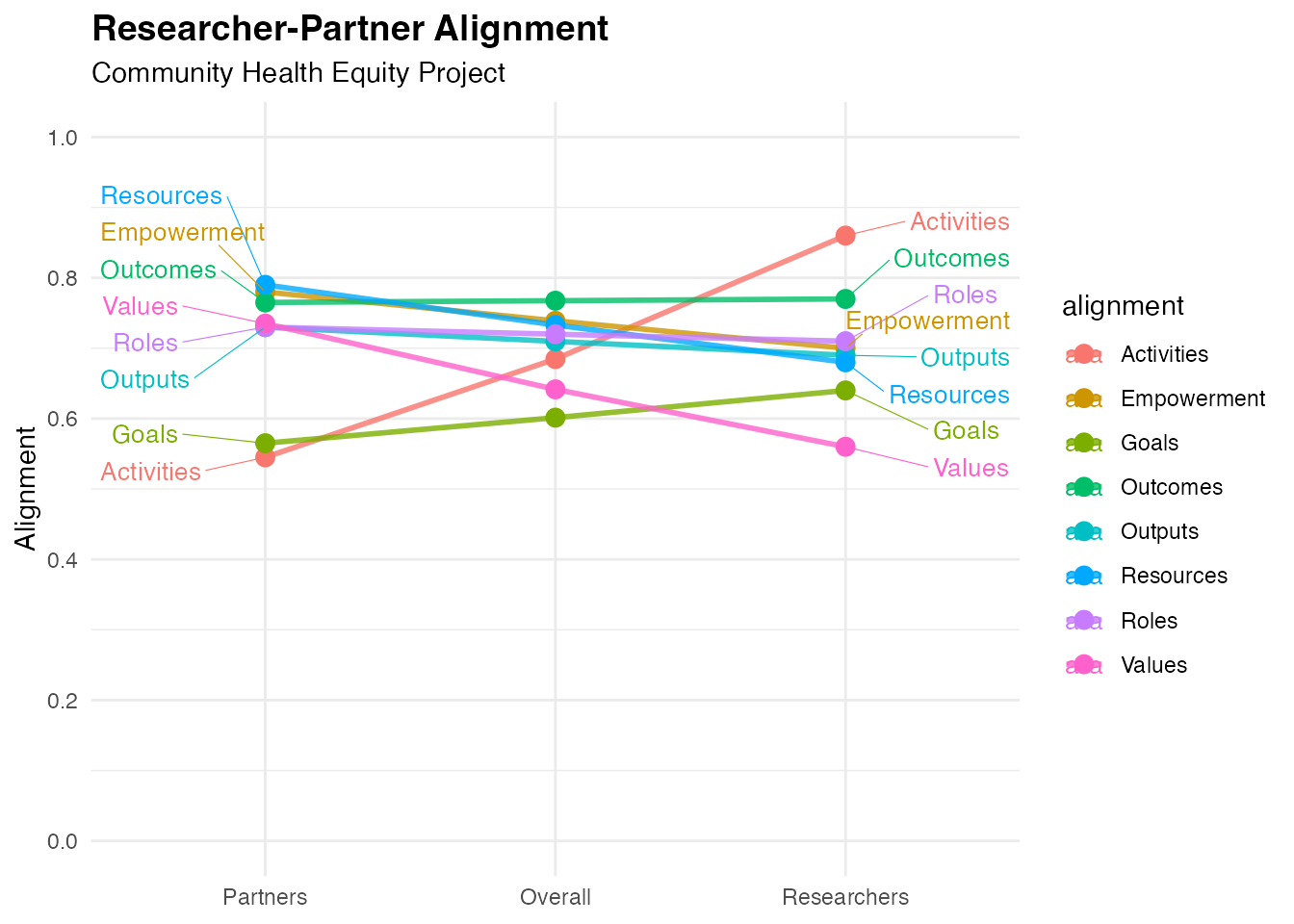
Complete Workflow Example
Here’s a complete workflow analyzing all four dimensions for a single project:
# 1. Alignment
alignment_data <- generate_alignment_data()
alignment_results <- analyze_alignment(alignment_data)
alignment_plot <- visualize_alignment(alignment_results)

# 2. Cascade Effects
cascade_data <- generate_cascade_data()
cascade_results <- analyze_cascade(cascade_data)
#> Running full exact analysis (~450 expected edges).
cascade_plot <- visualize_cascade(cascade_results)

# 3. Dynamics
dynamics_data <- generate_dynamics_data()
dynamics_results <- analyze_dynamics(dynamics_data)
dynamics_plot <- visualize_dynamics(dynamics_results)

# 4. Indicators
indicators_data <- generate_indicators_data()
indicators_plot <- visualize_indicators(indicators_data)

# Display alignment as example
print(alignment_plot)
#> Warning: Removed 1 row containing missing values or values outside the scale range
#> (`geom_line()`).
#> Warning: Removed 1 row containing missing values or values outside the scale range
#> (`geom_point()`).
#> Warning: Removed 1 row containing missing values or values outside the scale range
#> (`geom_text_repel()`).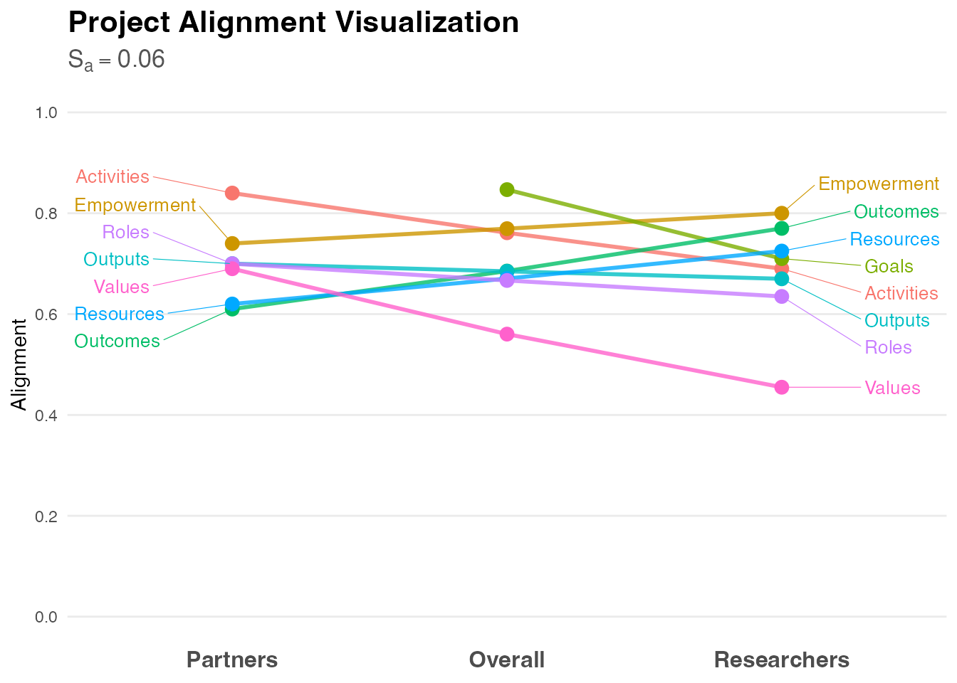
Interpreting Results
Alignment Scores
- 0.80-1.00: Strong alignment; shared vision well-established
- 0.60-0.79: Moderate alignment; some areas need attention
- Below 0.60: Low alignment; significant discussion needed
Cascade Scores
Higher scores indicate information and power successfully distributed across network degrees, suggesting sustainable community impact.
Preparing Your Own Data
Each analysis function expects data in specific formats. Use the
generate_*_data() functions as templates:
# Examine expected structure
str(generate_alignment_data())
#> 'data.frame':    144 obs. of  3 variables:
#>  $ alignment: chr  "Goals" "Goals" "Goals" "Goals" ...
#>  $ role     : chr  "researcher" "researcher" "researcher" "researcher" ...
#>  $ rating   : num  0.74 0.73 0.91 0.88 0.53 0.81 0.67 0.55 0.73 0.76 ...
str(generate_cascade_data())
#> 'data.frame':    1 obs. of  9 variables:
#>  $ cascade_d1_people_1_1: int 5
#>  $ cascade_d1_people_2_1: int 2
#>  $ cascade_d2_people_1_1: int 3
#>  $ cascade_d2_people_2_1: int 2
#>  $ cascade_d2_stats_1   : num 0.14
#>  $ cascade_d2_stats_2   : num 0.23
#>  $ cascade_d3_people    : int 1
#>  $ cascade_d3_stats_1   : num 0.07
#>  $ cascade_d3_stats_2   : num 0.12
str(generate_dynamics_data())
#> 'data.frame':    103 obs. of  4 variables:
#>  $ domain   : chr  "Contexts" "Contexts" "Contexts" "Contexts" ...
#>  $ dimension: chr  "Challenge" "Challenge" "Challenge" "Challenge" ...
#>  $ salience : num  0.4 0.6 1 0.2 0.8 1 0.2 0.6 0.8 0.4 ...
#>  $ weight   : num  0.84 0.84 0.78 1 0.84 0.95 1 1 0.9 0.95 ...
str(generate_indicators_data())
#> 'data.frame':    7 obs. of  2 variables:
#>  $ indicator: chr  "Community Partners" "Engagement Hours" "Individuals Served" "Infrastructure Tools" ...
#>  $ value    : int  6 3 14 0 10 9 16
Next Steps
- See
?analyze_alignmentfor detailed parameter descriptions - Explore
?visualize_alignmentfor customization options - Review individual function documentation for each dimension
- Consult the CEnTR*IMPACT framework report for theoretical foundations
References
Price, J. F. (2024). CEnTR*IMPACT: Community Engaged and Transformative Research – Inclusive Measurement of Projects & Community Transformation (CUMU-Collaboratory Fellowship Report). Coalition of Urban and Metropolitan Universities. https://cumuonline.org/wp-content/uploads/2024-CUMU-Collaboratory-Fellowship-Report.pdf
Wallerstein, N., & Duran, B. (2010). Community-Based Participatory Research Contributions to Intervention Research: The Intersection of Science and Practice to Improve Health Equity. American Journal of Public Health, 100(S1), S40–S46. https://doi.org/10.2105/AJPH.2009.184036
Wallerstein, N., et al. (2020). Engage for Equity: A Long-Term Study of Community-Based Participatory Research and Community-Engaged Research Practices and Outcomes. Health Education & Behavior, 47(3), 380–390. https://doi.org/10.1177/1090198119897075